22Tutorial 10 - Performance metrics and pole placement
Question 01
A second order system has a rise time of \(5~s\) and a overshoot of \(20 \%\). What is the settling time for this system?
Question 02
Consider a ship of length \(150~m\) and design speed \(18~knots\) with Nomoto parameters \(T'=3\) and \(K'=-1.2\). A control engineer has designed a heading autopilot with the following dimensional gains:
\(K_p = -1.0\)
\(K_d = -0.5\)
\(K_i = -0.1\)
Is the closed loop system stable? Use Routh-Hurwitz criteria to establish stability.
Question 03
Consider a ship of length \(120~m\) and design speed \(20~knots\) with Nomoto parameters \(T'=2\) and \(K'=-1\). You are tasked with designing an underdamped PD heading autopilot for this ship that must satisfy the following performance metrics:
Rise time of less than \(10~s\)
Settling time of less than \(20~s\)
What should be the values of the proportional and derivtive gains that achieve the limiting values of the performance metrics?
Question 04
Consider a ship of length \(100~m\) and design speed \(10~knots\) with Nomoto parameters \(T'=3\) and \(K'=-1\). For a PD heading autopilot with dimensional gains \(K_p = -1.0\) and \(K_d = -0.3\), determine the bandwidth of the closed loop system \(\Psi(s) / \Psi_d(s)\) and compare it with \(1 / T\). What can you infer?
Question 01 Solution
A second order system has a rise time of \(5~s\) and a overshoot of \(20 \%\). What is the settling time for this system?
Consider a ship of length \(150~m\) and design speed \(18~knots\) with Nomoto parameters \(T'=3\) and \(K'=-1.2\). A control engineer has designed a heading autopilot with the following dimensional gains:
\(K_p = -1.0\)
\(K_d = -0.5\)
\(K_i = -0.1\)
Is the closed loop system stable? Use Routh-Hurwitz criteria to establish stability.
Code
import numpy as npimport matplotlib.pyplot as pltdef solve_problem_02(): L =150 U =18*0.5144 Tprime =3 Kprime =-1.3 Kp =-1.0 Kd =-0.5 Ki =-0.1 T = Tprime * L / U K = Kprime * U / L a3 = T a2 =1+ K * Kd a1 = K * Kp a0 = K * Ki b1 = (a2*a1 - a3*a0) / a2 b2 =0 c1 = a0 c2 =0 d1 =0print(f"Routh Array")print(f"{a3:.3f}\t{a1:.3f}\n{a2:.3f}\t{a0:.3f}\n{b1:.3f}\t{b2:.3f}\n{c1:.3f}\t{c2:.3f}\n{d1:.3f}") roots = np.roots(np.array([a3, a2, a1, a0]))print("\nActual roots")print(f"{roots[0]:.4f}\n{roots[1]:.4f}\n{roots[2]:.4f}")solve_problem_02()
Consider a ship of length \(120~m\) and design speed \(20~knots\) with Nomoto parameters \(T'=2\) and \(K'=-1\). You are tasked with designing an underdamped PD heading autopilot for this ship that must satisfy the following performance metrics:
Rise time of less than \(10~s\)
Settling time of less than \(20~s\)
What should be the values of the proportional and derivtive gains that achieve the limiting values of the performance metrics?
Code
import numpy as npimport matplotlib.pyplot as pltdef solve_problem_03(): Tprime =2 Kprime =-1 L =120 U =20*0.5144 T = Tprime * L / U K = Kprime * U / L Kp = T * np.pi**2/ (400* K) Kd = (2* T /5-1) / Kprint(f"Kp: {Kp:.2f}, Kd:{Kd:.2f}")solve_problem_03()
Kp: -6.71, Kd:-97.18
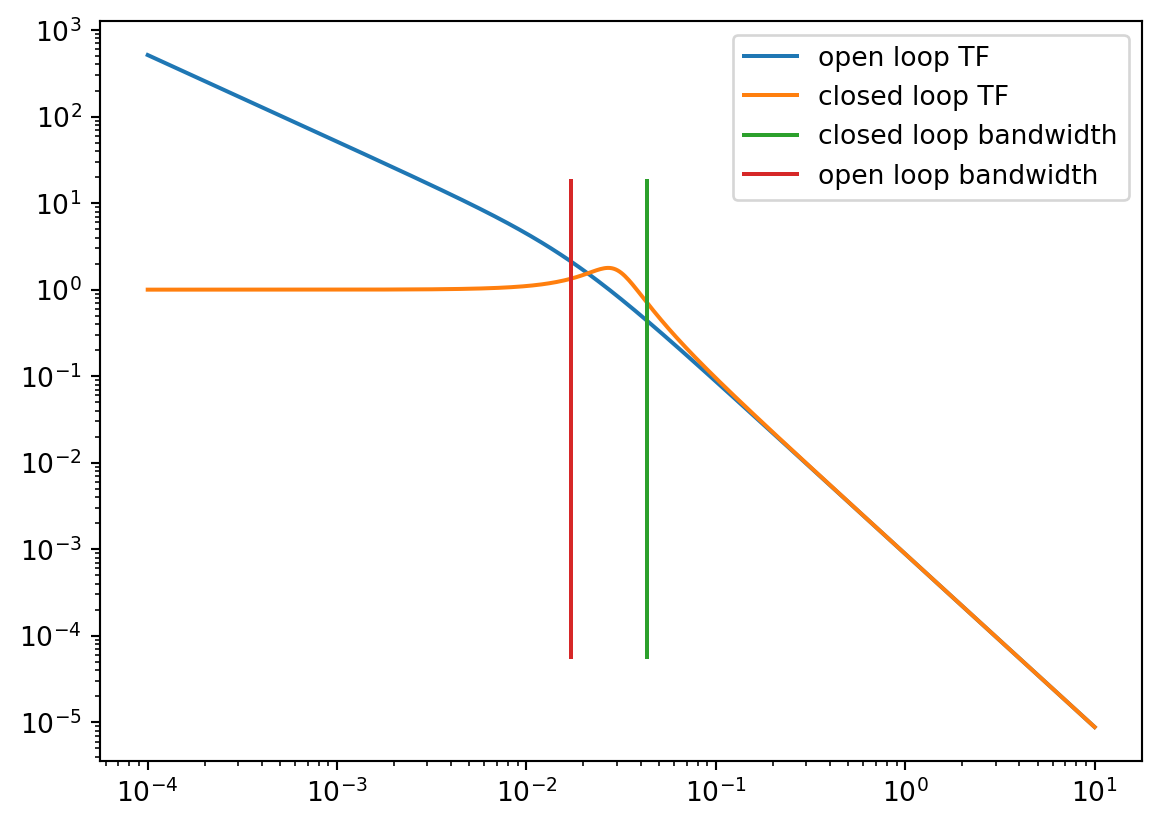
Question 04 Solution
Consider a ship of length \(100~m\) and design speed \(10~knots\) with Nomoto parameters \(T'=3\) and \(K'=-1\). For a PD heading autopilot with dimensional gains \(K_p = -1.0\) and \(K_d = -0.3\), determine the bandwidth of the closed loop system \(\Psi(s) / \Psi_d(s)\) and compare it with \(1 / T\). What can you infer?